Table of contents
🔗 Code available in this Colab
Introduction
In sequential recommendation, the goal is to predict the next item a user will engage with based on their historical interactions—such as views, clicks, or purchases. Whether it's shopping on Amazon or discovering videos on YouTube, the task remains the same: modeling user behavior over time to anticipate future actions. Transformer-based models like SASRec and its variants have proven highly effective for this, and are widely deployed in practice, powering systems such as Meta's Transducers or Pinterest’s PinnerFormer.

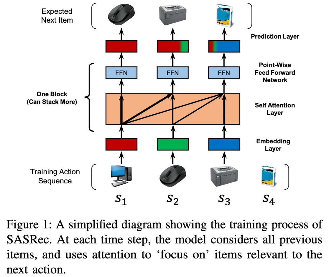
SASRec: Borrowing from language, adapting to catalogs
The SASRec architecture is essentially a causal language model —but instead of natural language tokens, it operates on items in the catalog. While originally formulated as a 0-1 classification task using the binary cross-entropy loss, recent works such as [Klenitskiy & Vasilev] and [Petrov & Macdonald] have shown that framing it as multi-class classification problem with cross-entropy loss achieves state-of-the-art results.
Now, in sequential recommendation, the item catalog plays the role of the vocabulary—but unlike words in a language model, this vocabulary is not fixed. It differs across platforms and lacks a shared structure. An item's representation is platform-dependent; for example, a movie's embedding on Netflix—shaped by its context and Netflix users—can differ significantly from its embedding on Hulu. This variability often necessitates platform-specific foundational models trained on their own interaction data.
Scalability Challenges and Techniques for Large Catalogs
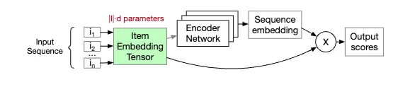
On curated platforms like Netflix or Hulu, where the catalog size is manageable, typically under 20,000 unique movies and shows, it's often sufficient to learn a d-dimensional embedding (commonly 128 or 256) for each item. However, the situation changes drastically as the number of items explodes into the 100s of millions, as is the case on platforms like Instagram, YouTube, and TikTok. In such massive catalogs, working directly with an embedding for each item becomes computationally prohibitive, in the forward pass and especially during the scoring phase while computing the loss.
Negative Sampling to speed up loss computation
Negative sampling is a widely used technique: rather than scoring every item in the catalog, it focuses on scoring only the target item(positive) alongside a small set of randomly sampled negatives. This technique has been around since the early days of large-scale recommendation, notably in two-tower models like YouTubeDNN, and in works such as Sampling Bias Correction and Google-MixedNegSampling. The same sampling ideas appear in sequential recommenders like PinnerFormer, and are further discussed in the Sampling for SeqRec survey.
That said, even with these computational gains, negative sampling still requires storing and maintaining the full item embedding table, which becomes a bottleneck at scale.
Codebook/Tokenization Techniques
In sequential recommendation, training requires computing the loss at every position in the transformer's output sequence—a process that becomes increasingly expensive with longer context lengths. To mitigate this, recent methods focus on reducing the effective vocabulary size. Notably, methods like TIGER and RecJPQ introduce a form of tokenization by constructing codebooks that group similar items together. This reduces the number of unique items that need to be scored, making training more efficient.
ID based vs. Metadata based Models
Here, it's important to highlight a key detail about architectures like SASRec: these are what we call ID-only methods—meaning they rely solely on the item IDs that each user has interacted with, learning embeddings for each item from scratch, without using any metadata such as titles, descriptions, categories, or genres. While one could argue this approach misses out on potentially useful information, these models still perform remarkably well. In fact, they remain state-of-the-art (SoTA) when dealing with large-scale, private item catalogs, as shown in the recent Meta paper: Trillion-Parameter Sequential Transducers for Generative Recommendations.
On the other end of the spectrum are metadata-driven approaches like UniSRec, GPT4Rec, and CALRec, which leverage pretrained language models. These works serialize catalog items into natural language. For example, instead of representing an item like the movie Toy Story as an ID-to-embedding mapping, they use a textual representation such as:
Title: Toy Story, Year: 1995, Genre: Family/Adventure, Summary: Woody, a good-hearted cowboy doll who belongs to a young boy named Andy …
This natural language representation enables the use of powerful pretrained language models, improving generalization—especially in cold-start or sparse data settings. Also by operating directly on text, they scale effectively as they don’t require an item embedding table.
Dataset and typical preprocessing steps
Dataset
We’ll walk through an example using the Amazon Industrial and Scientific dataset (2018), specifically the core-5 dataset. This dataset has been reduced using the k-core filtering method, ensuring that each remaining user and item has at least 5 reviews.
We'll be working with two JSON files and their corresponding fields:
- Product metadata
https://mcauleylab.ucsd.edu/public_datasets/data/amazon_v2/metaFiles2/meta_Industrial_and_Scientific.json.gzThis file contains metadata about ASINs (Amazon Standard Identification Numbers). Each row includes:
-
asin -
title -
brand -
main category -
price
-
- Reviewer-ASIN interactions
https://mcauleylab.ucsd.edu/public_datasets/data/amazon_v2/categoryFiles/Industrial_and_Scientific.json.gzThis file captures interactions between reviewers and ASINs. Each row contains:
-
reviewerID -
asin -
unixReviewTime -
overall(the reviewer’s rating for this product on a scale of 1 to 5)
-
Processing the Product Metadata File
The product metadata file contains essential information about each product (ASIN), such as the title, brand, category, and price. Key preprocessing steps include:
- Duplicate ASIN Checks: Ensuring there are no repeated entries for the same ASIN.
- Data type consistency: Verifying that each column contains values of consistent and same data type (e.g., all prices as a float, titles as a string).
Processing the Reviewer-ASIN Interaction File
This Reviewer-ASIN interactions file contains records of user interactions with products. Each row includes the reviewer ID, product ASIN, rating, and timestamp. Our main preprocessing are:
- Data type consistency: As with the product metadata, we ensure that each column has a consistent data type.
- Chronological Sorting: A crucial step for any sequential modeling task is to preserve the temporal order of interactions. We sort the dataframe first by
reviewerID, and then byunixReviewTimein ascending order. This ensures that each reviewer's history is properly ordered. - Deduplication of Interactions: An often-overlooked issue in recommendation datasets is duplicated interaction rows. If not removed, these duplicates can lead to inflated performance metrics, as models learn to "memorize" and repeat items.
- ✨ Important Note: This is a conservative deduplication—we only remove exact duplicates with the same user, item, timestamp, and rating. We do not remove valid repeated interactions, such as a user reviewing the same product at different times or giving different ratings at the same time.
sci5 = pd.read_json('Industrial_and_Scientific_5.json',\
										 lines=True)
sci5 = sci5[['reviewerID', 'asin', 'unixReviewTime', \
						 'overall']]
df_withdup = sci5.copy()

# Sort the dataframe by reviewerID and unixReviewTime
df_withdup = df_withdup.sort_values(by=['reviewerID', \
						 'unixReviewTime']).reset_index(drop=True)

# Drop exact duplicates based on key fields
df_dedup = df_withdup.drop_duplicates(subset=['reviewerID', \
					 'unixReviewTime', 'asin', 'overall'])

print(df_withdup.shape)
percentage_duplicates = (1 - len(df_dedup) / len(df_withdup)) * 100
print(f"Percentage of duplicates: {percentage_duplicates:.2f}%")
print(df_dedup.shape)

--------------------------------
(77071, 4)
Percentage of duplicates: 6.04%
(72419, 4)
Here’s the code that applies all the preprocessing steps described above.
The ASINs in the reviewer–item interaction file define the item catalog or corpus—this is the pool of items from which recommendations are generated.
Evaluation metrics and splits
In sequential recommendation the typical evaluation strategy is the leave-one-out split, where the final item in a user's sequence is held out as test data.
Leave one out(LOO) split
As seen in the figure below, in the leave one out (LOO) split, the final item in a user's interaction sequence is held out for testing and all preceding items are used for training.
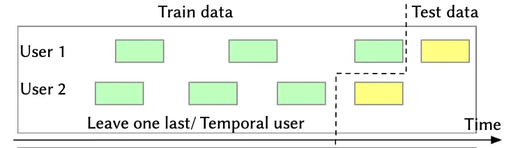
Note: For hyperparameter tuning, it's common to reserve a small randomly sampled subset of users typically around 5% for validation. For these users, the first items are used for training, the item serves as the validation target item, and the final item is used for testing. For the remaining 95% of users we use the first items for training and the last item for testing.
DatasetDict({
    train: Dataset({
        features: ['reviewer_id', 'text'],
        num_rows: 11039
    })
    validation: Dataset({
        features: ['reviewer_id', 'ptext', 'text', 'seen_asins', 'asin', 'asin_text'],
        num_rows: 512
    })
    test: Dataset({
        features: ['reviewer_id', 'ptext', 'text', 'seen_asins', 'asin', 'asin_text'],
        num_rows: 11039
    })
})Here’s the code that creates the leave-one-out (LOO) splits as Hugging Face datasets. A few notes on the key fields:
-
seen_asinsin the validation and test splits is a list of ASINs corresponding to the reviewer’s history (containing and items respectively) -
ptextis a prefix constructed from the reviewer’s purchase history, ending withNext item:to indicate where a language model should begin generating.
Below is a customer's purchase history on Amazon, listed in chronological order (earliest to latest).
 Each item is represented by the following format: Title: <item title> Category: <item category> Brand: <item brand> Price: <item price>.
 Based on this history, predict only one item the customer is most likely to purchase next in the same format.
### Purchase history:
Title: Herbal Choice Mari Natural Toothgel, Cinnamon & Baking Soda; 3.4floz Glass. Brand: Nature's Brands. Category: Health & Personal Care. Price: $14.47
Title: Pac-Kit by First Aid Only 25-450 Cotton Tipped Applicator with 6" Wooden Shaft (Bag of 100). Brand: First Aid Only. Category: Industrial & Scientific. Price: Unknown
### Next item:
-
asin_textis the target ASIN text:
Title: Litmus pH Test Strips, Universal Application (pH 1-14), 2 Packs of 100 Strips. Brand: LabRat Supplies. Category: Industrial & Scientific. Price: Unknown -
asinis the target ASIN string e.g.B00S730YWG
Baselines
Performance is typically evaluated using metrics such as nDCG@k, Recall@k, and Mean Reciprocal Rank (MRR). For @k metrics, each method needs to return k candidate items; in the experiments, I’ll use k = 10.
I’ll now discuss 4 training-free baseline heuristics that any capable recommender system should aim to outperform:
- Random from Corpus: Recommend k items randomly (without replacement) from the item catalog.
- Popularity-Based Sampling: Recommend k items (without replacement) from the catalog, with probabilities proportional to each item’s total # of ratings.
- Repeat Last Seen Items: Recommend the last k ASINs the user interacted with. If the user has interacted with fewer than k items, the remaining candidates are filled using popularity-based recommendations.
- Text-Based Last Item Similarity (e.g., BM25): Retrieve k items similar to the last item the user interacted with by comparing item text using fast text-based retrievers like BM25.
These baselines are also implemented and evaluated in the accompanying Colab notebook. For the text-based item similarity baseline, I use the bm25s package. To measure metrics like nDCG@k, Recall@k I’m using the ranx package.
from ranx import Qrels, Run, evaluate
import bm25s
import Stemmer

def get_qrels(dataset):
    '''
    Generates a ground truth dictionary (qrels) from the input dataset.
    Returns:
        A dictionary where keys are 'reviewer_id' and values are dictionaries
        mapping 'asin' to a relevance score of 1.
        Example: {'user_1': {'item_a': 1}, 'user_2': {'item_b': 1, 'item_c': 1}}
    '''
    qrels_dict = {}
    for row in dataset:
        reviewer_id = row['reviewer_id']
        asin = row['asin']
        if reviewer_id not in qrels_dict:
            qrels_dict[reviewer_id] = {}
        qrels_dict[reviewer_id][asin] = 1
    return qrels_dict

#BASELINE 2
def randrecs_popweighted(scimeta_corpus, dataset, item_popularity: pd.Series, k=5, seed=42):
    np.random.seed(seed)
    run_dict = {}
    all_asins = item_popularity.index.tolist()
    probabilities = item_popularity.values / item_popularity.sum()
    for row in dataset:
        reviewer_id = row['reviewer_id']
        sampled_asins = np.random.choice(all_asins, size=k, replace=False, p=probabilities)
        scores = {asin: item_popularity.get(asin, 0) for asin in sampled_asins}
        run_dict[reviewer_id] = scores
    return run_dict

#BASELINE 4
def textbased_lastsimilar(dataset, retriever, asin_dict, asins_compact, k = 5):
    queries_flat = [asin_dict[seen[-1]] for seen in dataset['seen_asins']] # text of last asin for each reviewerID
    query_tokens = bm25s.tokenize(queries_flat, stopwords="en")
    res, scores = retriever.retrieve(query_tokens, k=k) # has shape (len(dataset), k) for both res and scores
    run_dict = {}
    for i in range(len(dataset)):
        reviewer_id = dataset['reviewer_id'][i]
        asin_indices = res[i]
        asin_scores = scores[i]
        asins = asins_compact.iloc[asin_indices]['asin'].tolist()
        run_dict[reviewer_id] = {asin: score for asin, score in zip(asins, asin_scores)}
    return run_dict

# Demo usage
scimeta_corpus = pd.read_json('scimeta_corpus.json', \
															orient='records', lines=True)
scimeta_corpus.columns = ['asin', 'Title', 'Brand',\
													'Category', 'Price']
k = 10
metrics = ["recall@10", "ndcg@10", "mrr"]
item_pop = df_withdup['asin'].value_counts()
qrels_test = Qrels(get_qrels(dataset_withdup['test']))
print("Qrels (test):")
print("-" * 30)

run_test_popweighted = Run(randrecs_popweighted(scimeta_corpus, \
											 dataset_withdup['test'], item_pop, k=k))
print("Popularity-Weighted Recommendations (test):")
print("-" * 30)
ans_popweighted = evaluate(qrels_test, run_test_popweighted, metrics)
print(ans_popweighted)
Results
| Baselines | Recall@10 | nDCG@10 | MRR |
|---|---|---|---|
| B1. Random from corpus | 0.0021 | 0.0009 | 0.0006 |
| B2. Popularity-weighted recs | 0.0072 | 0.0054 | 0.0048 |
| B3. Repeat Last Seen Items | 0.0470 | 0.0433 | 0.0421 |
| B4. Text-Based Last Item Similarity | 0.1400 | 0.0886 | 0.0723 |
The table above shows the performance of the four baselines on the dataset, without any item deduplication applied. We measure Recall@10, NDCG@10, and MRR, and observe that Text-based last item similarity performs the best, followed by Repeat Last Seen Items.
| Baselines on the deduplicated dataset | Recall@10 | nDCG@10 | MRR |
|---|---|---|---|
| B1. Random from corpus | 0.0017 | 0.0007 | 0.0005 |
| B2. Popularity-weighted recs | 0.0082 | 0.0065 | 0.0060 |
| B3. Repeat Last Seen Items | 0.0119 | 0.0074 | 0.0060 |
| B4. Text-Based Last Item Similarity | 0.1100 | 0.0571 | 0.0403 |
The table above presents the performance of the same four baselines on the dataset where duplicate reviewer-ASIN interactions have been removed from the recommendation lists. As a reminder, we removed interactions with identical reviewer ID, ASIN, timestamp, and rating—ensuring that only true duplicates were eliminated. We observe a performance drop across all three metrics. For the two best-performing methods, this drop is significant—ranging from 20% to 80% (see table below). This is a key aspect of the experimental design and should be clearly communicated in any reported results.
| Impact of item dedup on metrics | Recall@10 | nDCG@10 | MRR |
|---|---|---|---|
| B3. Repeat Last Seen | -74.79% | -82.93% | -85.67% |
| B4. Text-Based Last Similar | -21.39% | -35.53% | -44.24% |
Conclusion
In this post, we explored sequential recommenders—from ID-based models like SASRec and MetaTransducers to text-based approaches like UniSRec, GPT4Rec, and CALRec
We walked through key preprocessing steps, including item deduplication in reviewer-item sequences, and showed how even removing exact duplicates can lead to a significant drop in metrics.
We also introduced four simple, training-free baselines. Among these, Text-Based Last Item Similarity performed the best. In any case, trained models should aim to outperform all of these baselines.
In the next post, I’ll evaluate raw and fine-tuned LLMs on our processed Hugging Face datasetShow information for the linked content, following a query generation pipeline similar to GPT4Rec.
Stay tuned!
If you found this write-up useful in your work, please consider citing it as:
Acharya, Krishna. (Apr 2025). A Primer on Generative Recommendation: Part 1. krishnacharya.github.io. https://krishnacharya.github.io/posts/generative-recommendation-part-1/
or
title = {A Primer on Generative Recommendation: Part 1},
author = {Acharya, Krishna},
journal = {krishnacharya.github.io},
year = {2025},
month = {Apr},
url = {https://krishnacharya.github.io/posts/generative-recommendation-part-1/}
}