🔗 Code available at https://github.com/krishnacharya/nanoGenRec
Table of contents
Overview
In my previous post, we looked at sequential recommenders and their various types, from ID-based models like SASRec to fully text-based approaches such as GPT4Rec. We also formatted item interactions as a leave-last-item-out Hugging Face dataset, and evaluated four training-free baselines that any trained model should aim to beat. Among these, the last item text similarity baseline — which recommends the k items most similar to the user's last item text, performs the best.
In this post, I will build a fully text-based recommendation pipeline using a query generation and retrieval strategy inspired by GPT4Rec. We will use models from the LLaMA-3 family (1B, 3B, 8B) and fine-tune them on serialized Amazon review interaction data using the unsloth library. I demonstrate that even on a single GPU with 24GB VRAM (RTX A5000), and without any¹ hyperparameter tuning, we can achieve state-of-the-art results.
¹other than for selecting a generation strategy post training
Recommender Pipeline
The pipeline consists of three main steps:
- Serialize: Format each user’s item interaction history into a chronological text sequence using the item metadata.
- Finetune: Fine-tune a LLM on these user sequences.
- Serving: To predict the target ( item) prompt the model with the serialized history ( items). Generate k candidates, and retrieve the closest item for each of these using a classic text retriever like BM25.
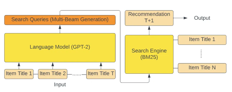
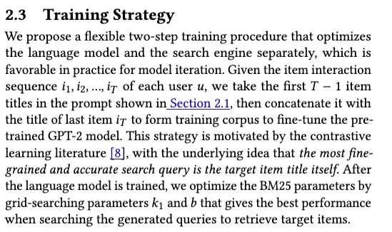
Despite extensive searching, I couldn't find an official codebase or reproduction of the GPT4Rec paper. My implementation reproduces many elements of their pipeline, with some key differences. First, I do not perform a grid search over the BM25 parameters k₁ and b; a recent Google paper (CALRec) also suggests this tuning step is not critical. Second, instead of GPT2 and full fine-tuning, I use LoRA to finetune 4-bit quantized LLaMA-3 models (1B,3B, 8B).
Serialize
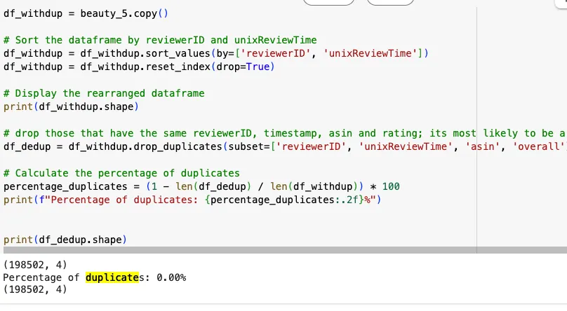
Similar to the GPT4Rec paper, we will use the core 5 Amazon beauty dataset and the corresponding metadata, both available at https://jmcauley.ucsd.edu/data/amazon/index_2014.html. In a previous post, I emphasized the importance of deduplicating user-item interaction rows to avoid inflated performance metrics. To address this, I applied a conservative deduplication strategy — removing only exact duplicates where the user, item, timestamp, and rating are all identical. I have created a Colab notebook to process this data here, which confirms that there are no exact duplicates.
DatasetDict({
train: Dataset({
features: ['reviewer_id', 'text'],
num_rows: 22363
})
validation: Dataset({
features: ['reviewer_id', 'ptext', 'text', 'seen_asins', 'asin', 'asin_text'],
num_rows: 1118
})
test: Dataset({
features: ['reviewer_id', 'ptext', 'text', 'seen_asins', 'asin', 'asin_text'],
num_rows: 22363
})
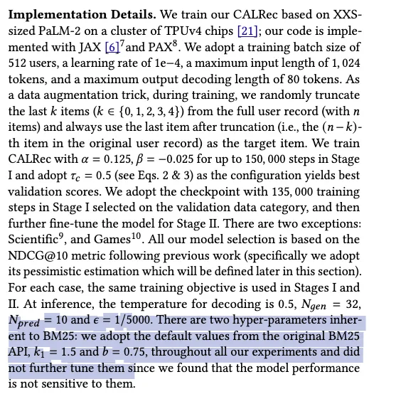
})Illustrated below in the left panel is the leave-one-out (LOO) split, the final item in each user’s interaction sequence is held out for testing, while the preceding items are used for training. For hyperparameter tuning, it's common practice to reserve a small, randomly sampled subset of users—roughly 5%—for validation. For these users, the first items are used for training, the item is used as the validation target, and the final item is used for testing.
Quick overview of the serialized data
Now let’s look into how the item history is serialized, using a single user as an example.
Suppose this user has rated the following 6 ASINs,
['B007IY97U0', 'B00870XLDS', 'B008MIRO88', 'B00BQYYMN0', 'B00GRTQBTM', 'B000052YU']The first 5 ASINs represent training items. We retrieve their titles and serialize this information into the user's training dataset under the text field as follows:
Below is a customer's purchase history on Amazon, listed in chronological order (earliest to latest).
Each item is represented by the following format: Title: <item title>
Based on this history, predict only one item the customer is most likely to purchase next in the same format.`
### Purchase history:
Title: 63cm Long Zipper Beige+pink Wavy Cosplay Hair Wig Rw157
 Title: MapofBeauty Long Wave Curly Hair Wig Full Wig for Women Long (Black)
 Title: MapofBeauty Cosplay Costume Long Curly Hair Wig Ladies Synthetic Wigs (White)
 Title: 32" 80cm Long Hair Heat Resistant Spiral Curly Cosplay Wig (Red Dark)
### Next item:
Title: MapofBeauty 28" 70cm Long Curly Hair Ends Costume Cosplay Wig (Brown)text field exampleFor the test dataset, the main field is ptext, which denotes the prefix/prompt text fed to the LLM. It ends with ### Next item:, signaling the model to generate text for the most likely next item.
Below is a customer's purchase history on Amazon, listed in chronological order (earliest to latest).
Each item is represented by the following format: Title: <item title>
Based on this history, predict only one item the customer is most likely to purchase next in the same format.`
### Purchase history:
Title: 63cm Long Zipper Beige+pink Wavy Cosplay Hair Wig Rw157
Title: MapofBeauty Long Wave Curly Hair Wig Full Wig for Women Long (Black)
Title: MapofBeauty Cosplay Costume Long Curly Hair Wig Ladies Synthetic Wigs (White)
Title: 32" 80cm Long Hair Heat Resistant Spiral Curly Cosplay Wig (Red Dark)
Title: MapofBeauty 28" 70cm Long Curly Hair Ends Costume Cosplay Wig (Brown)
### Next item: ptext field, the n-1 training items’ text is in the purchase history and generation must continue after next item.Notes on the other fields in the test & val datasets: seen_asins, asin, asin_text, text
seen_asins, asin, asin_text, text-
seen_asins:In both the validation and test splits, this field contains a list of ASINs representing the reviewer's interaction history.
- For validation, it includes the first n-2 items.
- For testing, it includes the first n-1 items.
-
asin: This is the target ASIN string that the model is expected to predict, e.g.B0CSTC4D13
-
asin_text: This is the serialized metadata for the target ASIN, such as its title, brand, category, and price. Example:
Title: MapofBeauty Beautiful Women's Flat Bang Long Wave Curly Wig (Black) -
text: We’ve already discussed this field in the training dataset. In the validation and test datasets it’s is used to compute next-token generation loss during evaluation of the LLM. Its not used for actual generation.Below is a customer's purchase history on Amazon, listed in chronological order (earliest to latest).
Each item is represented by the following format: Title: <item title> Category: <item category> Brand: <item brand> Price: <item price>.
Based on this history, predict only one item the customer is most likely to purchase next in the same format.### Purchase history:Title: 63cm Long Zipper Beige+pink Wavy Cosplay Hair Wig Rw157
Title: MapofBeauty Long Wave Curly Hair Wig Full Wig for Women Long (Black)
Title: MapofBeauty Cosplay Costume Long Curly Hair Wig Ladies Synthetic Wigs (White)
Title: 32" 80cm Long Hair Heat Resistant Spiral Curly Cosplay Wig (Red Dark)Title: MapofBeauty 28" 70cm Long Curly Hair Ends Costume Cosplay Wig (Brown)### Next item:Title: MapofBeauty Beautiful Women's Flat Bang Long Wave Curly Wig (Black)
Finetuning
For finetuning, we will use the Unsloth library, which has 4-bit quantized models for the LLaMA-3 family (1B , 3B, 8B). These models will be fine-tuned on the serialized Amazon training dataset, using the textShow information for the linked content field. I’m using a LoRA rank and alpha of 16, which results in approximately 11 million trainable parameters for the 1B model, 24 million for the 3B model & 42 million for the 8B model. The other finetuning parameters can be found in the corresponding YAML config files.
- https://github.com/krishnacharya/nanoGenRec/blob/main/ft_configs/llama1b_1024_beauty.yml
- https://github.com/krishnacharya/nanoGenRec/blob/main/ft_configs/llama3b_1024_beauty.yml
- https://github.com/krishnacharya/nanoGenRec/blob/main/ft_configs/llama8b_1024_beauty.yml
Note that I’m using an effective batch size of 16 (batch size of 4 with gradient accumulation steps of 4), this safely stays within the 24GB VRAM limit of my RTX A5000 GPU. I will now cover a few finer details of the fine-tuning process — feel free to skip if you're already familiar with standard LLM workflows.
Finetuning subtleties
- Adding an EOS token: this little snippet below is essential, without it the finetuned LLM struggles with sequence termination, leading to issues like run-on generations or poorly defined outputs.
def add_eos_to_text(example, tokenizer):
    return {"text": example["text"] + tokenizer.eos_token}

train_dataset = train_dataset.map(add_eos_to_text, fn_kwargs={"tokenizer": tokenizer})
eval_dataset = eval_dataset.map(add_eos_to_text, fn_kwargs={"tokenizer": tokenizer})
- Padding: during fine-tuning, pad tokens should be added to the right, after the EOS token. For the LLaMA 3 family, the special tokens can be found here, During generation, however, padding should be added to the left (as a prefix) — see this discussion for more context.
# During finetuning
tokenizer.padding_side = "right"
tokenizer.truncation_side = "left"

# During inference
tokenizer.padding_side = "left"
tokenizer.truncation_side = "left"- Context window limits & truncation: I cap the maximum context length at
1024tokens and, as shown in the code above, apply left-side truncation — discarding earlier interacted item text to preserve the most recent context. During generation, it's also important to account for the combined length of the prefix and themax_new_tokens, and truncate accordingly — more on that later.
Loss Curves and GPU Utilization
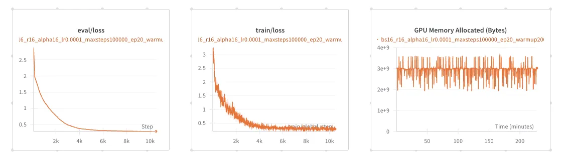
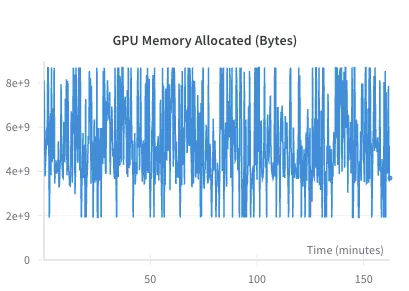
Finetuning LLaMA-3.2-1B takes roughly 3.5 hours, with training and validation loss stabilizing at a cross-entropy of around 0.28. Peak VRAM usage remains under 4GB, as seen in the third plot on the right.
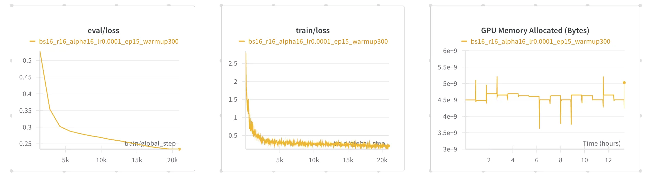
Finetuning LLaMA-3.2-3B takes about 12 hours, with training and validation cross-entropy loss stabilizing around 0.22. Peak VRAM usage stays below 5.5GB.
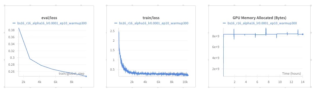
Finetuning LLaMA-3.1-8B takes 14 hours, with training and validation cross-entropy loss stabilizing around 0.24. Peak VRAM usage stays below 9GB.
Serving
Below is a customer's purchase history on Amazon, listed in chronological order (earliest to latest).
Each item is represented by the following format: Title: <item title>
Based on this history, predict only one item the customer is most likely to purchase next in the same format.`
### Purchase history:
Title: 63cm Long Zipper Beige+pink Wavy Cosplay Hair Wig Rw157
Title: MapofBeauty Long Wave Curly Hair Wig Full Wig for Women Long (Black)
Title: MapofBeauty Cosplay Costume Long Curly Hair Wig Ladies Synthetic Wigs (White)
Title: 32" 80cm Long Hair Heat Resistant Spiral Curly Cosplay Wig (Red Dark)
Title: MapofBeauty 28" 70cm Long Curly Hair Ends Costume Cosplay Wig (Brown)
### Next item: ptext field is fed to the finetuned LLM, generation continues after ### Next item:Evaluation recap
When evaluating performance, we typically measure metrics such as Recall@k, Mean Reciprocal Rank (MRR), and nDCG@k. The BM25 parameters are fixed to their default values, so the primary design choice lies in how we generate texts from the LLM. The GPT4Rec paper recommends using beam search with the number of beams set to k. Alternatively, we can employ sampling with temperature, which is the approach taken by the CALRec paper, though with additional refinements.
Generation + Search Strategies
- Beam Decoding + BM25 search: This strategy generates k sequences (beams), maintaining the k most probable sequences at each decoding step. For each of these k generated texts, we then search the BM25 index to find the closest item texts, resulting in k candidate ASINs. Implementation: generate_candidates_beam.py
- Temperature sampling + BM25 search :Unlike the sequential nature of beam search, temperature sampling allows for parallel generation. Here, we directly generate k sample texts from the LLM and then search the BM25 index to find the closest item texts, yielding k candidate ASINs. Implementation: generate_candidates_sampled.py
- Temperature Sampling + Modulated Search (CALRec): The CALRec paper proposes a more elaborate sampling + search. Instead of generating k=5 texts, they generate texts. These generated texts are then deduplicated and sorted by their log-likelihood generation scores. Finally, a combined score is calculated by modulating between the log-likelihood score and the BM25 score to determine the top k item scores.
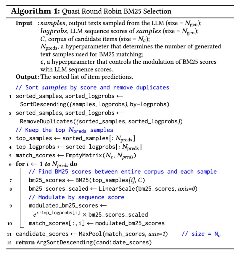
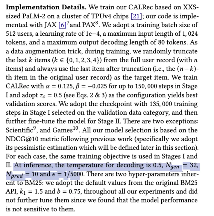
Note on implementation: Running CALRec's sampling and modulation search is expensive for two reasons: (1) it involves generating 32 completions per user, and (2) computing generation scores for each sample isn’t natively supported in Hugging Face — it requires recomputation, adding more latency. If you’d still like to explore this approach, here’s some starter code: generationscore_stepthru.py.
I will now cover a few subtleties details for generation — feel free to skip if you're already familiar with standard LLM inference.
Generation subtleties
For Hugging Face's generation config, I used the following settings: max_new_tokens=50 and num_return_sequences=5. Specifically, for beam search, num_beams=5, and for temperature sampling, I experimented with temperatures of 0.5, 0.2, and 0.1.
- Padding: during generation, padding should be added to the left (as a prefix) —see this discussion for more context.
- Context length & Truncation: During generation, it's also important to account for the combined length of the prefix and the
max_new_tokens, and truncate accordingly — as done in the code below.
tokenizer.padding_side = "left"
tokenizer.truncation_side = "left"
inputs = tokenizer(input_texts,
                   return_tensors="pt",
                   padding=True,
                   truncation=True,
                   max_length=model.max_seq_length - max_new_tokens
                  ).to(model.device)

input_ids = inputs.input_ids
attention_mask = inputs.attention_mask
input_seq_len = input_ids.shape[1] # Length of the tokenized input prefix/prompt

generation_config = {
    "max_new_tokens": max_new_tokens,
    "num_return_sequences": num_return_sequences,
    "temperature": temperature,
    "do_sample": True,
    "top_k": 50,
    "top_p": 0.95,
    "pad_token_id": tokenizer.pad_token_id,
    "eos_token_id": tokenizer.eos_token_id,
    "output_scores": False,
    "return_dict_in_generate": False
}

generated_outputs_ids = model.generate(
    input_ids=input_ids,
    attention_mask=attention_mask,
    **generation_config,
    use_cache=True # not optimized
)
Results
Generation strategy selection
To choose the generation strategy, I first measured the performance of each strategy on the validation dataset. The table on the right records the Recall@5, nDCG@5 metrics and Mean Reciprocal Rank (MRR) obtained with the finetuned Llama-3.2-1B model.
Beam search yields the best performance for all the three metrics. Among the sampling strategies, a temperature of 0.2 is the best, with deviations towards both lower (more greedy) and higher (more stochastic) temperatures resulting in a decline in the metrics.
| Strategy | Recall@5 | nDCG@5 | MRR |
|---|---|---|---|
| Beam Search | 0.054 | 0.033 | 0.026 |
| Temp 0.5 | 0.011 | 0.007 | 0.006 |
| Temp 0.2 | 0.012 | 0.009 | 0.008 |
| Temp 0.1 | 0.006 | 0.006 | 0.005 |
Test metrics
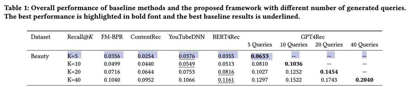
Given the promising performance of beam search, I proceeded to generate 5 target item texts for each user in the test dataset. Interestingly, the results in the table below shows that the last item similarity baseline performs remarkably well — even outperforming the Recall@5 of all four trained models in the GPT4Rec paper (FM-BPR, ContentRec, YouTubeDNN, and BERT4Rec)
| Metric | Last Item Similarity Baseline | Llama-1B | Llama-3B | Llama-8B |
| Recall@5 | 0.043 | 0.04534 (+5.44%) | 0.06519 (+51.60%) | 0.06814 (+58.47%) |
| nDCG@5 | 0.023 | 0.02687 (+16.83%) | 0.04003 (+74.04%) | 0.04232 (+84.00%) |
| MRR | 0.016 | 0.02086 (+30.38%) | 0.03184 (+99.00%) | 0.03390 (+111.88%) |
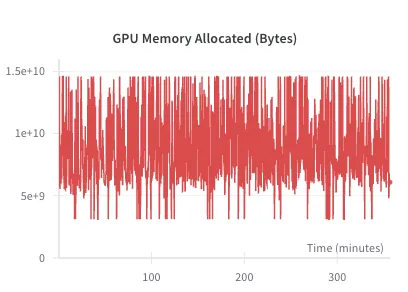
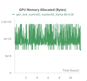
Generation time and GPU utilization
From left to right, the figures illustrate the VRAM usage for the 1B, 3B, and 8B parameter models during generation, respectively. Notably, the current inference pipeline (for which I'm using Hugging Face) uses more VRAM than finetuningShow information for the linked content and takes a couple of hours for generation. This is a stark contrast to Last Item text similarity, which completes in just 5 minutes and offers competitive performance across metrics.
Therefore, for practical deployment with a large user base, a tiered approach is beneficial. We could use the Last Item Similarity baseline as a fast initial filter for users, reserving the more computationally intensive 3B and 8B models for scenarios demanding higher recommendation quality.
Also, while distributed inference can reduce overall generation time, our main concern in retrieval settings is per-user generation speed. To address this, I believe the vLLM library’s optimized KV caching could offer significant speedups, and I plan to explore this integration in the future.
Conclusion
In this post, we built a fully metadata-based recommender system using an LLM for query generation and retrieval. We fine-tuned LLaMA-3 models (1B, 3B, 8B) with LoRA on Amazon review data, achieving state-of-the-art results on a single 24GB GPU without hyperparameter tuning.
Among the various generation and search strategies discussed, beam search performed the best. Additionally, the Llama-8B model outperformed the rest, showing double-digit percentage improvements (58-111%) across Recall@5, nDCG@5, and MRR metrics when compared to both the text-based item similarity and GPT4Rec models.
Our benchmarking of VRAM usage during finetuning and generation revealed that generation is a significant bottleneck. Consequently, real-time deployment requires optimized KV caching to increase per-user query generation speed and distributed inference to reduce total processing time.
Acknowledgements
I’m very grateful for the compute resources used in these experiments, provided by Simian — a GPU workstation set up by Prof. Jacob Abernethy and maintained by Tyler LaBonte, a fellow PhD student and total MVP.
If you found this write-up useful in your work, please consider citing it as:
Acharya, Krishna. (May 2025). A Primer on Generative Recommendation: Part 2. krishnacharya.github.io. https://krishnacharya.github.io/posts/generative-recommendation-part-1/
or
title = {A Primer on Generative Recommendation: Part 2},
author = {Acharya, Krishna},
journal = {krishnacharya.github.io},
year = {2025},
month = {May},
url = {https://krishnacharya.github.io/posts/generative-recommendation-part-2/}
}